Numerical Solution of Nonlinear Equations

A system of nonlinear equations is a system of equations comprising at least one nonlinear equation. As no analytical solution can be found in the majority of nonlinear systems, we have to approach those systems numerically, for example by Bisection Method or Newton method. However, Python enables the use of numerical solvers available in its libraries. Those solvers are ready to be implemented with no additional knowledge required. In this chapter, we will draw on sympy library. It could be installed by the command pip install sympy.

Numerical Solution of a Single Nonlinear Equation

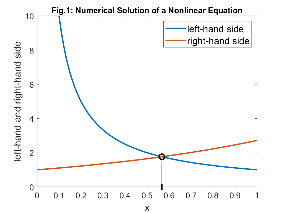
Take, for instance, the equation 1/x = exp(x), see Fig.1. We look for a value of x that fulfills the given equation.

    import sympy as sm
    
    x = sm.Symbol("x", real=True)
    equation = sm.Eq(1 / x, exp(x))
    init_val = 0.5
    solution = sm.nsolve(equation, x, init_val)
    print(solution)

If the program runs correctly, it prints the solution, approximately 0.5671. We may assign the result to the variable x, in case we need to work with that value later on.

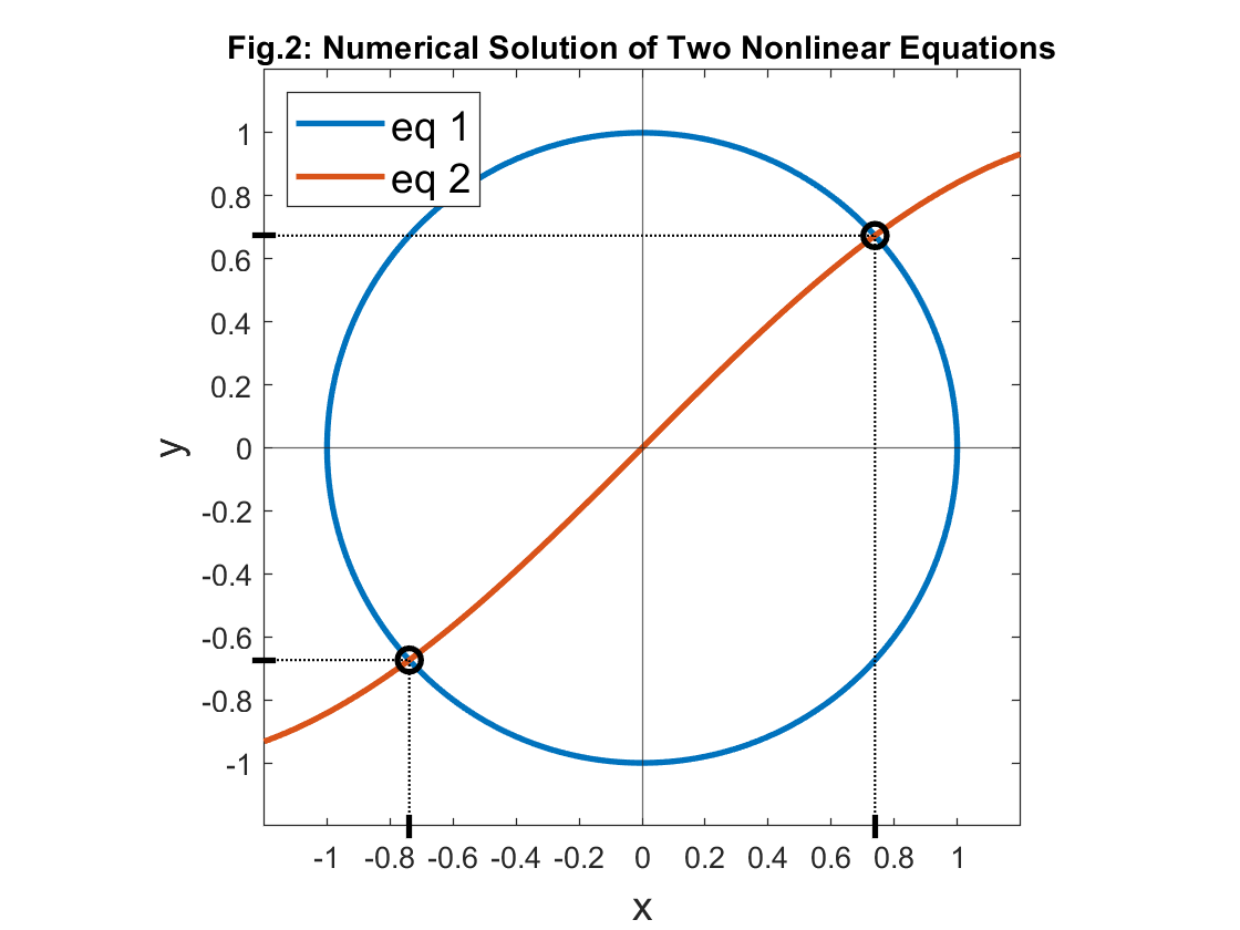
   x = solution

Numerical Solution of Two Nonlinear Equations

Similarly, nsolve enables solving systems of two or more nonlinear equations. For example, let’s find the the intersections of a unit circle placed at the origin of the coordinate system and a simple sine wave, in the form of equations eq1 and eq2, see Fig.2.

    from sympy import Symbol, Eq, nsolve
    
    x = Symbol("x", real=True)
    y = Symbol("y", real=True)
    unknowns = [x, y]
    
    eq1 = Eq(x ** 2 + y ** 2 - 1, 0)
    eq2 = Eq(y - sin(x), 0)
    equations = [eq1, eq2]

    init_vals = [1, 1]

    sol = nsolve(equations, unknowns, init_vals)
    print(sol)

If the program runs correctly, it prints the solution, approximately 0.7391 and 0.6736. Again, we may assign the result to the variables x and y, in case we need to work with them later on.

   x, y = sol

In case we choose the initial guess, for example, [-1, -1], the program find the other solution, corresponding to values -0.7391 and -0.6736.

Illustration on an Engineering Example

In this section, we will solve a system of four equation containing four unknowns, originating from an engineering problem (Problem 15-6b in Chemical Engineering I, chapter Chemical Reactors).

Note that this problem deals with a design calculation, that is, we know both inlet and outlet parameters and the task is to find the number of reactors in a cascade of reactors in order to attain the required cummulative conversion of the input material.

Snippet of Source Code

First, we declare intermediate results from the problem 15-6a.

    from sympy import Symbol, Eq, nsolve

    nuA, nuB, nuC = -2, 1, 1  # stoich coeffs
    k_plus = 5.0  # m3/kmol/h
    k_minus = 0.3125  # m3/kmol/h
    V0 = 6.2745  # m3
    cA0, cB0, cC0 = 1.50, 0.0, 0.0  # kmol/m3
    cAN, cBN, cCN = 0.433, 0.533, 0.533  # kmol/m3
    tau_dash = 0.062745  # h
    zetaAN = 0.711

Now, we will perform the first iteration of the calculation, that is, we will calculate the cumulative conversion of N-1 reactor, with N denoting the last reactor in the cascade. This “backward-going” approach is advantageous as we avoid the need of solving a quadratic equation where the uknown is the cumulative conversion, possibly leading to the problem regarding which retured value is relevant for the task.

# Balance of A in the last reactor (N) in the cascade
cAN_1 = cAN - nuA * (k_plus * cAN ** 2 - k_minus * cBN * cCN) * tau_dash

cAN_2= Symbol("cAN_2", real=True)
cBN_1 = Symbol("cBN_1", real=True)
cCN_1 = Symbol("cCN_1", real=True)
zetaAN_1 = Symbol("zetaAN_1", real=True)

# Equations concering (N-1)th reactor
eq1 = Eq(cAN_2 - cAN_1 + \
    nuA * (k_plus * cAN_1 ** 2 - k_minus * cBN_1 * cCN_1) * tau_dash, 0)
eq2 = Eq(cAN_1, cA0 * (1 - zetaAN_1))
eq3 = Eq(cBN_1, cB0 - nuB / nuA * cA0 * zetaAN_1)
eq4 = Eq(cCN_1, cC0 - nuC / nuA * cA0 * zetaAN_1)
equations = [eq1, eq2, eq3, eq4]

unknowns = [cAN_2, cBN_1, cCN_1, zetaAN_1]

init_vals = [cAN_1, cBN, cCN, zetaAN]
sol = nsolve(equations, unknowns, init_vals)
cAN_2, cBN_1, cCN_1, zetaAN_1 = sol
print(zetaAN_1)

The value of cummulative conversion in the (N-1)th reactor should be 0.640. Given that this value is positive, we must analogously solve these equations in multiple iterations.